

Fluids#
A wave on shallow water
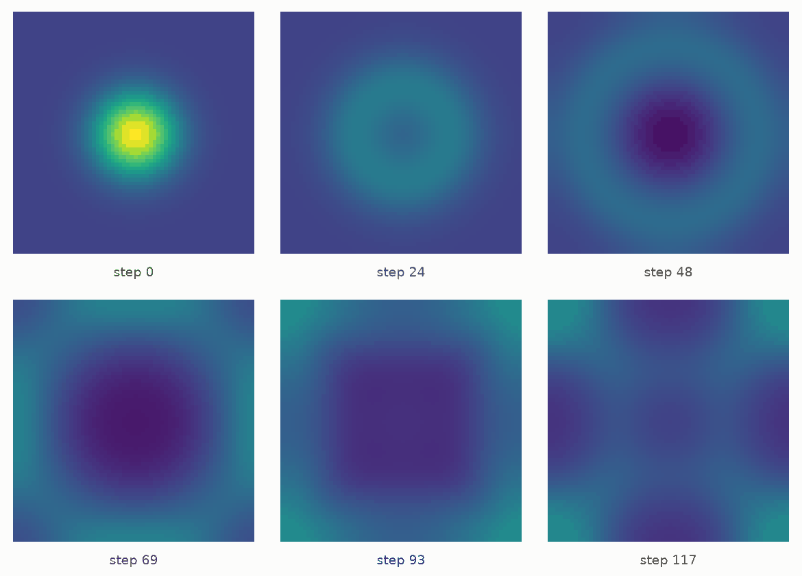
A pond has a raised mound of water in the middle. Under gravity the mound collapses and rings of waves travel out.
The shallow-water equations describe this with the depth h and the flow (hu, hv), and they conserve water: the
total of h never changes. This notebook steps them on a 2-D grid and prints that total as the check.
Time: ~5 min · Runs on: CPU (same code on GPU) · You need: hawk, NumPy and matplotlib; read first: hawk in your domain
Colab or Kaggle: run this first cell (it installs the packages and downloads the helper files this notebook uses). Elsewhere it only checks the imports.
import sys, pathlib
sys.path.insert(0, str(pathlib.Path.cwd().parent / "_shared"))
from nb_helpers import gpu_available, on_device, plot_style, show, to_numpy, xp
plot_style()
The pond’s words#
Say the vocabulary first. The pond is described by the depth h and the two momenta hu and hv; the step needs the gravity g and lam, the time step over the cell size. Declare them once as a KernelKind; the step below is written in these names.
from hawk import Param, Scalar
from hawk.ext import DATA_ONLY, KernelKind


class Water(KernelKind, slug="water"):
    h: Scalar               # depth of the water
    hu: Scalar              # momentum along x
    hv: Scalar              # momentum along y
    lam: Param              # time step over cell size
    g: Param                # gravity
    guard = DATA_ONLY

Water
__main__.Water
The step#
One finite-volume step with a Rusanov flux (also called local Lax-Friedrichs). Across each of a cell’s four faces the
flux is the mean of the two cells’ fluxes, minus a times the jump between them, where a is the faster signal speed
of the two, |flow| + sqrt(g h). The flux of the depth is the flow; the fluxes of the flow carry the momentum and the
pressure g h^2 / 2. The cell then loses what leaves through its faces. Grid["row", "col":width] sizes row at run time (row=N) and fixes col; the last axis declared, col, is the fastest (consecutive lanes, so coalesced on a GPU and SIMD on a CPU). The domain wraps around, so the first and last
rows and columns are neighbours; the if/else picks the wrapped index. The kernel writes three outputs, one per field.
The scheme is first order and diffusive: it smears the waves, and it is the simple, robust choice. Production codes use
the same flux with a higher-order reconstruction. Units: g = 1, a cell is 1 wide, still water is 1 deep, and the
step lam = dt / dx is 0.35. The scheme is stable while lam * (a_x + a_y) <= 1; the run checks the stricter
lam * (max(|u|, |v|) + sqrt(g h)) < 0.5 at every step.
The helpers are plain functions the kernel calls; the kernel itself assumes the grid has as many rows as columns (the row
wrap uses width).
import numpy as np
import eagle
import hawk
import hawk.math as m
from hawk import Grid, Mutable, Param, Scalar


def push(h, p, g):
    """Momentum flux along its own direction: p^2 / h plus the pressure g h^2 / 2."""
    return p * p / h + 0.5 * g * h * h


def speed(h, p, g):
    """The fastest signal along that direction: the flow plus the wave speed sqrt(g h)."""
    return m.abs(p / h) + m.sqrt(g * h)


def rusanov(f_left, f_right, u_left, u_right, a):
    """The flux across a face: the mean of the two fluxes, minus a times the jump."""
    return 0.5 * (f_left + f_right) - 0.5 * a * (u_right - u_left)


def swe_kernel(width):
    @Water
    def swe_step(lane: Grid["row", "col":width], h, hu, hv, lam, g,
                 h_new: Mutable[Scalar], hu_new: Mutable[Scalar], hv_new: Mutable[Scalar]):
        i, j = lane.row, lane.col
        if i == 0:
            n = i + (width - 1)
        else:
            n = i - 1
        if i == width - 1:
            s = i - (width - 1)
        else:
            s = i + 1
        if j == 0:
            w = j + (width - 1)
        else:
            w = j - 1
        if j == width - 1:
            e = j - (width - 1)
        else:
            e = j + 1
        he, hue, hve = h.at(row=i, col=e), hu.at(row=i, col=e), hv.at(row=i, col=e)
        hw, huw, hvw = h.at(row=i, col=w), hu.at(row=i, col=w), hv.at(row=i, col=w)
        hn, hun, hvn = h.at(row=n, col=j), hu.at(row=n, col=j), hv.at(row=n, col=j)
        hs, hus, hvs = h.at(row=s, col=j), hu.at(row=s, col=j), hv.at(row=s, col=j)
        # east and west faces carry the x flow, south and north the y flow
        a_e = m.max(speed(h, hu, g), speed(he, hue, g))
        a_w = m.max(speed(hw, huw, g), speed(h, hu, g))
        a_s = m.max(speed(h, hv, g), speed(hs, hvs, g))
        a_n = m.max(speed(hn, hvn, g), speed(h, hv, g))
        h_new = h - lam * (rusanov(hu, hue, h, he, a_e) - rusanov(huw, hu, hw, h, a_w)
                           + rusanov(hv, hvs, h, hs, a_s) - rusanov(hvn, hv, hn, h, a_n))
        hu_new = hu - lam * (rusanov(push(h, hu, g), push(he, hue, g), hu, hue, a_e)
                             - rusanov(push(hw, huw, g), push(h, hu, g), huw, hu, a_w)
                             + rusanov(hu * hv / h, hus * hvs / hs, hu, hus, a_s)
                             - rusanov(hun * hvn / hn, hu * hv / h, hun, hu, a_n))
        hv_new = hv - lam * (rusanov(hu * hv / h, hue * hve / he, hv, hve, a_e)
                             - rusanov(huw * hvw / hw, hu * hv / h, hvw, hv, a_w)
                             + rusanov(push(h, hv, g), push(hs, hvs, g), hv, hvs, a_s)
                             - rusanov(push(hn, hvn, g), push(h, hv, g), hvn, hv, a_n))
    return eagle.deploy(swe_step)


def mound(width):
    """Still water of depth 1 with a smooth raised mound in the middle."""
    y, x = np.mgrid[0:width, 0:width]
    h = 1.0 + 0.4 * np.exp(-((x - width / 2) ** 2 + (y - width / 2) ** 2) / (width / 6) ** 2)
    return h, np.zeros_like(h), np.zeros_like(h)


N, LAM, G = 64, 0.35, 1.0
step = swe_kernel(N)
state = mound(N)
out = step.run(h=state[0], hu=state[1], hv=state[2], lam=LAM, g=G, row=N)
sorted(out)
['h_new', 'hu_new', 'hv_new']
Check one step against NumPy#
The same step with np.roll for the neighbours. The three outputs must agree to rounding.
def numpy_step(h, hu, hv, lam, g):
    u = np.array([h, hu, hv])
    out = u.copy()
    for axis in (2, 1):                                  # columns carry hu, rows carry hv
        c, o = 3 - axis, axis                            # the flow along this axis, and the other one

        def flux(q):
            f = np.empty_like(q)
            f[0] = q[c]
            f[c] = q[c] ** 2 / q[0] + 0.5 * g * q[0] ** 2
            f[o] = q[c] * q[o] / q[0]
            return f

        right = np.roll(u, -1, axis)
        a = np.abs(u[c] / u[0]) + np.sqrt(g * u[0])
        a = np.maximum(a, np.roll(a, -1, axis - 1))
        face = 0.5 * (flux(u) + flux(right)) - 0.5 * a * (right - u)
        out -= lam * (face - np.roll(face, 1, axis))
    return out


TOL = 1e-12
want = numpy_step(*state, LAM, G)
err = max(np.abs(out[k] - w).max() for k, w in zip(("h_new", "hu_new", "hv_new"), want))
assert err < TOL, err
print(f"one step: largest difference from NumPy {err:.1e} < {TOL:g}")
one step: largest difference from NumPy 2.2e-16 < 1e-12
Run it and check the physics#
Feed the three outputs back in. Two sets of arrays take turns, and step.bind ties each direction to its arrays once:
forward reads set A and writes set B, backward reads B and writes A, and a step is one .launch(),
alternating the two. On a
GPU the fields stay on the device and copying a frame home is the only wait per frame (xp is CuPy there, NumPy
otherwise).
Once per frame the run checks the stability number. At the end three things are compared with what the equations say:
the total depth: water is neither made nor lost;
the symmetry: a round mound on a square grid must stay mirror-symmetric;
the energy
sum(0.5 (hu^2 + hv^2) / h + 0.5 g h^2): it must not grow. The scheme loses a little of it to its own numerical diffusion, and that loss is printed.
steps_per_frame, n_frames = 3, 40
A = [xp.array(a) for a in state]
B = [xp.empty_like(a) for a in A]
forward = step.bind(h=A[0], hu=A[1], hv=A[2], lam=LAM, g=G, row=N, h_new=B[0], hu_new=B[1], hv_new=B[2])   # A -> B
backward = step.bind(h=B[0], hu=B[1], hv=B[2], lam=LAM, g=G, row=N, h_new=A[0], hu_new=A[1], hv_new=A[2])  # B -> A
launches, sets, which = (forward, backward), (A, B), 0


def energy(h, hu, hv):
    return float((0.5 * (hu ** 2 + hv ** 2) / h + 0.5 * G * h ** 2).sum())


frames, volume, total_energy = [state[0]], [state[0].sum()], [energy(*A)]
worst_cfl = 0.0
for _ in range(n_frames - 1):
    for _ in range(steps_per_frame):
        launches[which].launch()
        which = 1 - which
    cur = sets[which]
    h, hu, hv = cur
    cfl = LAM * float((xp.maximum(abs(hu / h), abs(hv / h)) + xp.sqrt(G * h)).max())
    assert cfl < 0.5, cfl
    worst_cfl = max(worst_cfl, cfl)
    frames.append(to_numpy(cur[0]).copy())
    volume.append(float(cur[0].sum()))
    total_energy.append(energy(*cur))

volume, total_energy = np.array(volume), np.array(total_energy)
TOL_MASS = 1e-12
drift = np.abs(volume / volume[0] - 1.0).max()
assert drift < TOL_MASS, drift
print(f"water: total depth {volume[0]:.4f} at the start, {volume[-1]:.4f} at the end; "
      f"largest relative change {drift:.1e} < {TOL_MASS:g}")

final = frames[-1]
TOL_SYM = 1e-12
assert np.abs(final - final.T).max() < TOL_SYM
print(f"symmetry: largest difference between the depth and its mirror image {np.abs(final - final.T).max():.1e} < {TOL_SYM:g}")

assert np.all(np.diff(total_energy) <= 0.0), "the energy must not grow"
print(f"energy: {total_energy[0]:.2f} -> {total_energy[-1]:.2f}, a drop of "
      f"{100 * (1 - total_energy[-1] / total_energy[0]):.2f} % (the scheme's numerical diffusion); "
      f"largest stability number {worst_cfl:.2f} < 0.5")
water: total depth 4238.9709 at the start, 4238.9709 at the end; largest relative change 2.2e-16 < 1e-12
symmetry: largest difference between the depth and its mirror image 4.4e-16 < 1e-12
energy: 2205.27 -> 2200.68, a drop of 0.21 % (the scheme's numerical diffusion); largest stability number 0.42 < 0.5
The depth at the start and part-way through, and the total along the way. The colour scale starts at the mound’s full height, so the first panel is not clipped:
import matplotlib.pyplot as plt

fig, axes = plt.subplots(1, 3, figsize=(7.4, 2.6), constrained_layout=True)
for ax, f, title in zip(axes[:2], (frames[0], frames[n_frames // 2]), ("start", f"after {steps_per_frame * (n_frames // 2)} steps")):
    im = ax.imshow(f, vmin=0.9, vmax=1.4, cmap="viridis")
    ax.set_title(title); ax.set_xlabel("x (cells)")
axes[0].set_ylabel("y (cells)")
fig.colorbar(im, ax=axes[:2], shrink=0.8, label="depth h")
axes[2].plot(volume / volume[0] - 1.0, lw=1.2)
axes[2].set_ylim(-1e-9, 1e-9)
axes[2].set_xlabel("frame"); axes[2].set_title("total depth, change")
show()


A bigger pond, when a GPU is there#
The same kernel with a wider grid. Where the data lies decides where the kernel runs: NumPy arrays on the host, CuPy
arrays on the GPU. So the fields are handed over as device arrays and come back as device arrays; the check against NumPy
copies them home first. To choose a side yourself, use step.host.run(...) or step.device.run(...): the device plan takes NumPy
arrays, uploads them, runs on the GPU and brings the result home.
if gpu_available():
    big = 1024
    big_step = swe_kernel(big)
    sb = mound(big)
    got = big_step.run(h=xp.asarray(sb[0]), hu=xp.asarray(sb[1]), hv=xp.asarray(sb[2]), lam=LAM, g=G, row=big)
    assert on_device(got["h_new"]), "the result is a device array: the kernel ran on the GPU"
    ref = numpy_step(*sb, LAM, G)
    err = max(np.abs(to_numpy(got[k]) - w).max() for k, w in zip(("h_new", "hu_new", "hv_new"), ref))
    assert err < TOL, err
    print(f"{big} x {big} on the GPU (result is a device array): largest difference from NumPy {err:.1e}")
else:
    print("no GPU here; the grid stays at", N, "x", N)
1024 x 1024 on the GPU (result is a device array): largest difference from NumPy 2.2e-16
The animation#
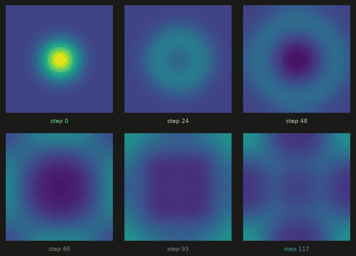
The last cell writes the depth frames as a looping GIF, one for a light page and one for a dark page; the page shows the file written when the notebook last ran.
import matplotlib.pyplot as plt
from anim import frame_of, write_anim
from themed_figure import DARK, LIGHT


def render(theme, field, label):
    pal = LIGHT if theme == "light" else DARK
    fig = plt.figure(figsize=(2.6, 2.8), dpi=80, facecolor=pal["bg"])
    ax = fig.add_axes([0.04, 0.12, 0.92, 0.84])
    ax.axis("off")
    ax.imshow(field, vmin=0.9, vmax=1.4, cmap="viridis", interpolation="nearest")
    fig.text(0.5, 0.04, label, ha="center", fontsize=9, color=pal["sub"])
    return frame_of(fig, pal["bg"])


for theme in ("light", "dark"):
    movie = [render(theme, f, f"step {k * steps_per_frame}") for k, f in enumerate(frames)]
    for name, size in write_anim(movie, "shallow_water_" + theme).items():
        print(name, f"{size / 1e3:.0f} kB")
shallow_water_light.gif 859 kB
shallow_water_dark.gif 849 kB
What just happened#
One kernel with three outputs advanced depth and flow together;
.atread the four neighbours, with theif/elsechoosing the wrapped index, and a Rusanov flux crossed each face.One step matched NumPy to rounding.
The total depth stayed fixed, the mound stayed mirror-symmetric, and the energy fell slightly, as a first-order scheme’s diffusion makes it.
Next#
Orbits shows a state vocabulary for a different domain.