Run your first kernel

Write one line of math, compile it once, and run it unchanged on the CPU or a GPU.

Time: ~5 min · Runs on: CPU, GPU switch · You need: NumPy (and CuPy, only if you have a GPU)

A kernel is a plain Python function decorated @hawk.kernel: each parameter’s type annotation says what role it plays for every sample.

import hawk
from hawk import Mutable, Param, Scalar


@hawk.kernel
def scale(x: Scalar,              # a per-sample input
          a: Param, b: Param,     # a shared constant: one value for the run
          y: Mutable[Scalar]):    # an output plane the body assigns
    y = a * x + b


scale

<Kernel scale slots=4>

hawk.artifact.build compiles it for a chosen target — "host" means the CPU alone, no GPU or eagle involved:

import pathlib
import tempfile

import hawk.artifact

work_dir = pathlib.Path(tempfile.mkdtemp())
hawk.artifact.build(scale, work_dir, targets=("host",));

hawk.load loads the compiled artifact and hawk.run runs it directly:

import numpy as np

host_kernel = hawk.load(work_dir, "scale")
x = np.linspace(0.0, 7.0, 8)
y = np.zeros(8)
hawk.run(host_kernel, x=x, a=2.0, b=1.0, y=y)
y

array([ 1.,  3.,  5.,  7.,  9., 11., 13., 15.])

That is the whole authoring surface for this kernel: declare the planes, write the arithmetic, build it, load/run it — no eagle and no GPU anywhere above.

The same kernel, wherever the data lives

eagle.deploy(scale) builds the same kernel for host and GPU through hawk’s cache (a rerun compiles nothing) and returns a plan — a small object that knows how to run this kernel on whatever array you hand it, NumPy or CuPy. The hidden cell below picks a GPU automatically when one is visible, and falls back to the CPU path otherwise — every tutorial in this family runs on CPU.

Show code cell source

Hide code cell source

import sys, pathlib as _pathlib
sys.path.insert(0, str(_pathlib.Path.cwd().parent / "_shared"))
from nb_helpers import DEVICE, plot_style, to_numpy, xp
plot_style()

import eagle

plan = eagle.deploy(scale, cache_dir=work_dir)
y_xp = plan.run(x=xp.asarray(x), a=2.0, b=1.0)
agrees = np.allclose(to_numpy(y_xp), y)
print("DEVICE:", DEVICE, "| y matches the CPU run:", agrees)

DEVICE: cpu | y matches the CPU run: True

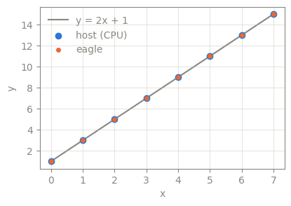
Same x, run on the host above and through eagle.deploy here — the numbers agree. One plot makes it visible:

Show code cell source

Hide code cell source

import matplotlib.pyplot as plt

fig, ax = plt.subplots(figsize=(4.5, 3))
ax.plot(x, y, color="#898781", lw=1.5, zorder=1, label="y = 2x + 1")
ax.scatter(x, y, color="#2a78d6", s=36, zorder=2, label="host (CPU)")
ax.scatter(x, to_numpy(y_xp), color="#eb6834", s=16, zorder=3, label="eagle")
ax.set_xlabel("x"); ax.set_ylabel("y"); ax.legend(frameon=False)
ax.grid(alpha=0.4)
plt.show()

What just happened

• A kernel’s parameter annotations declare its planes (Scalar, Param, Mutable[...]); the body is ordinary arithmetic over them.

• hawk.artifact.build + hawk.load/hawk.run compile and run a kernel on the host alone, with no eagle, no GPU, and no manifest involved.

• eagle.deploy(kernel) builds the same kernel for every target once and runs it wherever its data lives — a NumPy array on the CPU, a CuPy array on the GPU — so one plan serves both without a second code path.

Try this

In the build/run cells above, change b=1.0 to b=0.0 and re-run all three cells: the line now passes through the origin, and nothing else about the kernel changes.

Next

Arguments and shapes — pick the right plane type for a vector, a matrix, or a quaternion, and see how a batch of samples is laid out in memory. Deeper: Interoperability for every detail of how a plane binds to a NumPy/CuPy/Torch array.