The graph model: eagle.Graph

A real step is rarely one kernel. It is a propagation, then a diagnostic, then maybe a branch that only some runs take, and two pieces of work that have nothing to do with each other and could happen at the same time. eagle.Graph is where you write that down once and let eagle run it: as a captured CUDA graph on the GPU, or as an ordered run of host launches on the CPU. Same object, same calls, either way.

You add nodes. You never draw the edges between them: eagle reads which arrays each node touches and works the ordering out for itself. That is the one idea to carry through the page.

Note

New to the pieces? Build a step as a graph: eagle.Graph builds everything below step by step. GraphPipeline is unchanged: it is still the right tool when you want to record opaque callables yourself.

Your first graph

import numpy as np
import eagle
from eagle.graph import opaque

x, y, z = np.zeros(8), np.zeros(8), np.zeros(8)

g = eagle.Graph()
g.add_node(opaque(lambda: np.multiply(x, 2.0, out=y), reads={"x": x}, writes={"y": y}),
           name="double")
g.add_node(opaque(lambda: np.add(y, 1.0, out=z), reads={"y": y}, writes={"z": z}),
           name="shift")
g.build()
g.launch()

add_node takes a node; a plan launch is added with add(bound_plan) (a BoundPlan from plan.bind(...)). build() looks at where the planes live (numpy means the CPU, cupy means the GPU), derives the edges, refuses anything unsafe and lowers the graph. launch() runs it, launch(n) runs it n times. Every method returns the graph, so a build reads as one chain.

Nodes

Plan launches

Graph.add(bound, name=...) appends one BoundPlan. Its planes are the arrays you bound it over, and each plane’s role in the kernel (read, write, or both) tells eagle how the node touches it. A plane that would have to be copied before the launch (a non-contiguous or sample-major array) is refused: a graph needs to see the very array you hold, so pass a contiguous one.

Fork and join

Graph.add_group([branch, branch, ...]) is a stage: the branches may run at the same time, and the next node waits for all of them. A branch is a plan, a node, or a list of them (run in order inside the branch).

g.add_group([left_plan, right_plan], names=["left", "right"])

On the GPU the branches are captured as siblings, so the device can overlap them. On the CPU they run one after another in add order, and the result is the same, because branches that could race are refused (below).

Conditionals

The conditionals you already know work in a graph, written the way you always wrote them: eagle.skippable(step, guard) and eagle.repeat_while(step, guard, max_iters), handed to add_node.

guard = eagle.SkipGuard.nonzero(flag)
g.add_node(eagle.skippable(opaque(refine, reads={"x": x}, writes={"x": x}), guard),
           name="refine")

The step can be a node (an opaque op, with its planes declared), bound_plan.launch (its planes are then read off the plan) or any other zero-argument callable. A callable on its own has no declared planes, so only the guard’s own array takes part in the ordering; prefer one of the first two. A conditional holds one step: nesting one inside another, or a tuple of parts as the loop body, is refused for now.

Reductions

eagle.reduce(x, out, op="sum") is a node that adds up (or takes the "max" of, or the "all" of) a 1-D plane into a one-element plane. It reads x and writes out, so a node that produced x is ordered before it and a node that reads out after it, with nothing for you to declare. A floating-point "sum" always adds in the same fixed order, so the answer does not change with the number of CPU threads and the CPU and the GPU agree bit for bit; Same bits, every time: reductions has the details.

total = np.zeros(1)
g.add_node(eagle.reduce(energy, total), name="total")

Your own code in the graph: three tiers

eagle.graph.opaque(fn, reads=..., writes=...) wraps any zero-argument callable: a cupy elementwise kernel, a torch op, a host closure. You declare which arrays it touches; eagle still works out the edges, and the conflict check covers what you declared. The declaration says which planes, never which edges. Name the planes with a dict (reads={"x": x}) and they show up by name in every message and picture. Name every plane the node touches: an array it touches but you did not declare is invisible to the conflict check and to the reverse pass.

Give a node name="model" and it is that label in g.schedule, in messages and pictures, and in vjps={"model": ...} (below).

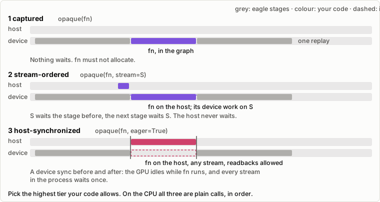
How it runs on the GPU is one keyword, and the ladder below says what waits where. Take the highest tier your code allows:

Spelling	What runs	Ordering
opaque(fn)	captured: replayed with the graph, also inside groups, conditionals and until_done steps. fn must not allocate.	the graph’s edges
opaque(fn, stream=S)	fn on the host every launch, its device work on S (a torch, CuPy or Warp stream, or a handle)	S waits the stage before, the next stage waits S; the host never waits
opaque(fn, eager=True)	fn on the host every launch, any stream, host readbacks allowed	a device sync before and after

g.schedule names each stage capture, eager_stream or eager_host, and print(g) tags the node [stream], [host] or [child]. On the CPU every tier is a plain call, in order (a stream= node is listed as [stream: cpu runs eagerly]).

What S’s work reads must stay alive until it ran: with torch, call tensor.record_stream(S) on a tensor you made inside fn. eagle.frameworks.jax.node(fn, reads=..., writes=...) builds a stream= node for a JAX step and keeps JAX’s results alive for you.

A graph your framework captured. eagle.graph.child(owner, reads=..., writes=...) inserts a torch.cuda.CUDAGraph (captured with keep_graph=True) or a warp.Graph as one node. eagle keeps owner alive and refuses a launch after owner.reset() or a re-capture; rebuild the eagle graph then. Do not replay the framework graph yourself while an eagle launch of it is in flight. On the CPU, call the model in an opaque.

Once per step of a stepping loop. eagle.until_done([model, plan], ...) runs a captured opaque or a child in list order once per step, over the whole batch. The plan takes one step per launch (steps=1); the node must never write a finished sample (pass terminated= and read it). A stream or host node cannot run inside the loop’s one device graph: call runner.run() with max_steps=k, then your code, in your own loop.

Gradients through your code. eagle.diff.reverse(g.record, seeds, vjps={"model": vjp}) runs vjp(primals, cotangents) -> {read name: gradient} in place of the node, host-synchronized; your model’s own parameter gradients are yours to accumulate.

Weights. Bind a Table plane to eagle.interop.import_buffer(param): one zero-copy buffer, so the optimizer’s in-place step is the refresh. Update weights after launch() returns (or synchronize() first), never between enqueue and synchronize. A launch after param.data = ... is refused by name: bind the tensor the optimizer updates.

How the edges are found

For every pair of nodes eagle asks, on your own arrays, whether they share a byte:

Edge	Meaning
RAW	data flows: read after write. The earlier node writes what the later one reads. This is the data flow, and the only kind a reverse pass follows.
WAR	must wait to overwrite: write after read. The later node overwrites what the earlier one read.
WAW	same output: write after write.

The test is stride-aware. Two column views of one (N, w) matrix do not overlap, a view of the tail of an array overlaps the array. It is exact up to a work cap and conservative past it: when in doubt eagle says overlap, which can only add an edge or refuse a graph, never miss a conflict. Scalars passed by value carry no edges.

g.edges() returns them as Edge(src, dst, plane, kind), indices into g.node_labels(); edge.meaning gives the plain-words reading above. It works before build() too.

What is refused

Each of these is a message that names what to change:

• Siblings that race. Two branches of one group where one writes what the other touches. The message names both nodes and both planes, so you can give each branch its own plane or put them in one branch.

• Copy-bound planes (see above), at add.

• Derivative kernels. A vjp/jvp kernel enters a graph only through eagle.diff, never directly.

• A graph that mixes host and device planes, or a backend= that disagrees with where the planes live.

• An empty graph, a second build, adding to a built graph.

• A conditional that is already another graph’s.

Build, launch, and what you get

build(backend=None) infers the backend from the planes (backend="cpu" or "gpu" states it). On the GPU it captures once (the captures counter moves by one, so does graph_builds); launch(n) then replays. enqueue(n) replays without waiting and synchronize() waits, exactly as on GraphPipeline; on the CPU enqueue is launch. g.backend is "gpu", "cpu" or None before the build, and g.schedule says how each stage runs ("capture" on the GPU, "work_share" or "branch_tasks" on the CPU, see below).

CPU schedules

On the CPU a stage runs one of two ways, and build picks per stage:

• "work_share": the stage’s nodes run one after another, each spread over the whole thread team. This is the right shape when a node has enough samples to keep every core busy, and it is the schedule of every plain (non-fork) stage.

• "branch_tasks": the independent branches of a fork/join stage run at the same time, each branch’s nodes in order on one thread, in a single native call that releases the GIL. This is the right shape for small batches (the control and MPC regime), where a team barrier per node costs more than the node: on a typical 8-core machine eight 16-node branches over 1024 samples run several times faster this way.

The choice is a fixed rule, not a heuristic: branch_tasks when the stage is a fork/join with at least two branches, the host team has at least two threads, there are at most 4096 samples (eagle._core.BRANCH_TASKS_MAX_SAMPLES), and every node is a plan launch; otherwise work_share. A branch holding a conditional or an opaque() Python callable always work-shares, because Python code cannot run inside the native branch runner. The rule is evaluated at build with the team size of that moment, and g.schedule reports the result.

Both schedules give bit-identical results to a serial run, and so does any thread count: a node is a per-sample kernel, so how its samples are cut across threads changes nothing, and a branch’s nodes always run in order. The executor opens one team region per run and never nests one: called from inside your own omp parallel region it runs in place on the calling thread. In C++ the same rule is eagle::exec::resolve and the branch runner is eagle::exec::runHostBranches (see API reference — host).

Using one graph from several threads

Distinct graphs run at the same time without any care. One graph shared by several threads is for one caller at a time: build, launch and enqueue hold a non-blocking guard, and a second thread entering while one is in flight gets eagle.Busy (“another call is still running on this Graph; give each thread its own Graph, or wait for it”). It is never queued behind the first and never handed a half-built state. The flag is a C++ atomic (eagle/util/Busy.h), so this holds on free-threaded Python too. Looking at a graph (below) takes no guard and never gets in the way.

Choosing fused or split kernels: dispatch=

A hawk kernel can declare a dispatch group with policy="auto": a switch over a per-sample selector. dispatch= on eagle.Graph.build() and eagle.simulate() says how those groups run. None (the default) keeps every group the author declared and decides the "auto" ones by measurement: the model starts fused, counts how many samples take each branch and, every 16 steps, splits the group into one kernel per branch when that is predicted to be at least 15 % faster (and fuses it again when the gain falls under 5 %). A policy name ("switch", "segmented", "predicated") or a {group: policy} dict forces the "auto" groups; a group the author gave a policy is never overridden. A built graph is one fixed structure, so Graph.build takes "switch" and "predicated" only; the split is decided as a run goes, in eagle.simulate(). What was chosen is in graph.dispatch and result.report.dispatch.

Seeing your graph

Print it:

g.show()          # or print(g), or str(g)

eagle.Graph  4 nodes · 1 group · backend: cpu

  stage 0 work_share       ┌╌╌╌╌╌╌╌┐
                           ╎ seed  ╎
                           └╌╌╌┬╌╌╌┘
                               x
                         ┌─────┴─────┐
  stage 1 work_share ┌╌╌╌┴╌╌╌┐   ┌╌╌╌┴╌╌╌┐
                     ╎ left  ╎   ╎ right ╎
                     └╌╌╌┬╌╌╌┘   └╌╌╌┬╌╌╌┘
                         left_out    right…
                         └─────┬─────┘
                      ╭─ skip if guard ─╮
  stage 2 work_share  │ ┌╌╌╌╌╌╌┴╌╌╌╌╌╌┐ │
                      │ ╎   combine   ╎ │
                      │ └╌╌╌╌╌╌╌╌╌╌╌╌╌┘ │
                      ╰─────────────────╯

Each node is a box on its stage, the plane names sit under the node that writes them, a conditional is a frame carrying its label (skip if guard, repeat ≤ N), a dashed border marks an opaque node, and after build() each stage shows how it runs. The header line says what the graph is so far (and recorded once the graph records for a reverse pass). It works on the graph as it stands, built or not.

Draw it, with matplotlib (an optional extra: pip install "raptor-eagle[plot]"):

fig = g.plot()                    # a matplotlib Figure
fig.savefig("graph.png")

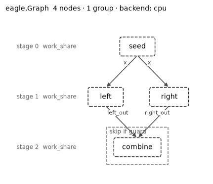
g.plot() on the graph above. Dashed boxes are opaque nodes, the dashed frame is the conditional, the labels on the arrows are the planes.

plot(ax=None, edge_labels=True, show_schedule=True) draws into your own axes if you pass one. The figure it makes is a plain matplotlib.figure.Figure (no pyplot state), so it is safe on a machine with no display.

For your own docs and tools there are two text formats:

print(g.to_mermaid())     # flowchart TD ... paste into a Markdown page
print(g.to_dot())         # Graphviz DOT

All four pictures come from one layout engine (C++, shared with the C++ graphs described in Seeing a graph from C++: eagle/graph), so they always agree.

Adding a kind of node

Plan launches, groups, conditionals and opaque ops cover most steps. A new kind of node (a reduction, say) is registered, not patched in:

from eagle.graph import register_node_kind, Node

register_node_kind("my_kind", reads=..., writes=..., lower_gpu=..., lower_cpu=...)
g.add_node(Node("my_kind", payload), name="mine")

reads/writes return (plane_name, array, role) tuples (that is what the edge derivation sees), lower_gpu returns what the capture loop runs and lower_cpu the host arm. Registering the same kind twice is fine; registering a different kind under an existing name is refused.

Where next

• Build a step as a graph: eagle.Graph: build, inspect and break a graph, hands on.

• Seeing a graph from C++: eagle/graph: print and lay out a C++ graph with the same engine.

• CUDA graphs: the C++ capture/replay machinery a GPU build lowers to.