

Profile your run#
Three numbers tell you where a run’s time went – compiling the kernel, running it, and bringing the result home – before you ever reach for a profiler.
Time: ~4 min · Runs on: CPU (GPU: this notebook picks it up automatically) · You need: Steps per launch
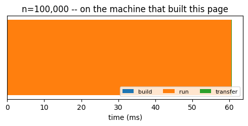
You will build the figure below: a build / run / transfer breakdown of your own run, on your own machine.
import time

DEVICE = "gpu" if gpu_available() else "cpu"
xp = xp_for(DEVICE)
print("running on", DEVICE)
running on cpu
The code: timing the three phases yourself#
RunReport (what eagle.until_done()’s runner hands back)
already carries build_s, the one-time graph-capture cost (zero on the
host, since there is no graph to build there). Wrapping the run itself in
time.perf_counter() and timing the step that brings the result home with
to_host gives the other two numbers, with no extra dependency.
import eagle
import hawk
from hawk import Mutable, Param, Scalar, Terminated


@hawk.kernel(steps="auto")
def oscillator(omega: Scalar, t_end: Param, dt: Param, terminated: Terminated,
               x: Mutable[Scalar], v: Mutable[Scalar], t: Mutable[Scalar]):
    x0, v0 = x, v
    x = x0 + dt * v0
    v = v0 - dt * omega * omega * x0
    t += dt
    terminated = t >= t_end


n = 1_000_000 if DEVICE == "gpu" else 100_000
planes = dict(x=xp.ones(n), v=xp.zeros(n), t=xp.zeros(n),
              omega=xp.linspace(1.0, 3.0, n), t_end=1.0, dt=1e-3)
runner = eagle.until_done(eagle.deploy(oscillator), max_steps=10_000, **planes)

t0 = time.perf_counter()
report = runner.run()
t1 = time.perf_counter()
x_home = to_numpy(planes["x"])      # the only step that actually moves data home
t2 = time.perf_counter()

build_s = report.build_s
run_s = max((t1 - t0) - build_s, 0.0)
transfer_s = t2 - t1
print(f"build: {build_s * 1e3:.2f} ms, run: {run_s * 1e3:.2f} ms, "
      f"transfer: {transfer_s * 1e3:.2f} ms")
print(f"launches: {report.launches}, steps: {report.steps}, "
      f"launches_by_k: {report.launches_by_k}")
build: 0.00 ms, run: 60.61 ms, transfer: 0.05 ms
launches: 16, steps: 1024, launches_by_k: {64: 16}
import matplotlib.pyplot as plt

fig, ax = plt.subplots(figsize=(5, 2.6))
segments = [
    ("build", build_s, "C0"), ("run", run_s, "C1"), ("transfer", transfer_s, "C2"),
]
left = 0.0
for label, width_s, color in segments:
    ax.barh(0, width_s * 1e3, left=left * 1e3, color=color, label=label)
    left += width_s
ax.set_xlabel("time (ms)")
ax.set_yticks([])
ax.set_title(f"n={n:,} -- on the machine that built this page")
ax.legend(loc="lower right", ncols=3, fontsize=8)
fig.tight_layout()
plt.show()
What just happened#
report.build_sis the one-time graph-capture cost What a graph is introduced; it is zero on the host team, since there is no graph to build there, and zero on any laterrunner.run()call that replays the same build.“run” is everything the loop itself did while it was out of Python’s hands – every launch, and every compaction or reorder
report.compactions/report.reorderscounts.“transfer” is only the last step: bringing the result home with
to_host. On the host team there is nothing to bring home (the arrays were already there), so it reads as zero; on the device it is a real device-to-host copy.
Why the first run is slower (GPU card)#
The build time above already shows this, just smaller: a kernel nothing has
compiled yet pays hawk’s build cost once. On the RK7(8) card, a cold run of
the eagle arms (eagle graph and eagle.simulate both deploy the
same hawk kernel) costs 3.36 s; the exact same kernel, rerun with a warm
cache – even in a new process – costs 527 ms. eagle.deploy and
eagle.until_done reuse hawk’s own build cache, so only the very first call
in a fresh environment pays the cold price; every later one, in this
notebook or a new process pointed at the same cache, is warm.
Useful FLOP/s vs. issued bytes/s#
Two different yardsticks for the same run, in the performance card’s own
words: useful FLOP/s counts only the steps of samples that are still
running – a sample that already finished contributes nothing, no matter how
it is computed. Issued bytes/s counts the bytes an arm’s own kernels
actually move, including the passes it makes over samples that already
finished. A kernel that compacts finished samples away can have low issued
bytes/s and still be fast; a plain kernel that always sweeps the whole batch
can issue a lot of bytes without doing much useful work. Both are also
reported as a fraction of the device’s own peak – the peaks device_props()
below reads off the hardware.
Looking inside the kernels#
The three numbers above come from Python; they don’t say how long each GPU kernel ran, or how many there were. Nsight Systems answers that from the outside, with no code changes:
nsys profile --stats=true python run.py
--stats=true prints a kernel-by-kernel summary table to the terminal once
the trace finishes – the same tool (with a longer flag list) the
performance card’s own kernel-only numbers come from. This needs a CUDA GPU
and nsys installed, so it is shown here rather than run.
Device properties – what useful FLOP/s/issued bytes/s are measured
against as a fraction of peak – come from the compiled extension itself,
read once per device:
if DEVICE == "gpu":
    props = eagle.device_props()
    print(f"{props.name} -- {props.sm_count} SMs, "
          f"fp64 peak is 1/{props.fp64_ratio:.0f} of this card's fp32 peak")
else:
    print("eagle.device_props() needs a CUDA GPU; skipped on this machine.")
eagle.device_props() needs a CUDA GPU; skipped on this machine.
Try this#
Drop max_steps to 100 and re-run: report.done turns False – the run
stopped at the cap, not because every sample finished – and the “run”
segment above shrinks with it.
Next#
Device properties and a two-plugin force manifest (how-to) –
device_props()combined with a two-plugin force manifest.Tutorials – the C++ track, if you want eagle’s own graphs and kernels with no Python in between.
deeper: Performance (“Method”) – the full accounting this page borrows from.