

A multi-kernel step, declaratively#
A physical step sometimes needs more than one kernel: advance the state,
derive a diagnostic from it, then decide whether to stop. This tutorial
builds that step two ways — one simulate call, then the same loop by hand,
piece by piece, so you can see (and reuse) what the call puts together.
Time: ~7 min · Runs on: CPU, GPU if visible (picked up automatically)
· You need: What a graph is (Plan.bind, GraphPipeline) and
Finished samples: compaction, reorder, and when not to (ActiveSet, compaction).
You will build: an ensemble of damped oscillators settling toward rest, and a plot of where each one’s energy ends up.
DEVICE = "gpu" if gpu_available() else "cpu"
xp = xp_for(DEVICE)
print("running on", DEVICE)
running on cpu
import numpy as np

import hawk
from hawk import Mutable, Param, Scalar, Terminated
from hawk.ext import Guard, Kind

from eagle import (
    ActiveSet, GraphPipeline, SkipGuard, compaction_body,
    deploy, repeat_while, simulate,
)
The one call#
simulate runs the kernels in list order, as one step. Pass the
arguments as you would call the kernels: an array gives each sample its
own value (x, v), a plain number is shared by every sample (omega,
zeta, dt, eps); energy, written by diagnostic, is allocated for
you. The step stops for a sample once event marks it, and the batch
stops when every sample has settled or after max_steps. Each launch
takes one step.
n = 20_000
x0 = np.random.default_rng(3).uniform(-1.0, 1.0, n)
result = simulate(kernels, x=xp.asarray(x0), v=xp.zeros(n),
                  omega=3.0, zeta=0.15, dt=0.01, eps=0.01,
                  max_steps=600, every=16)
n_settled = int(result.finished.sum())
print(result.status, f"after {result.steps} steps:",
      f"{n_settled} / {n} settled; allocated for you: {result.allocated}")
max_steps after 608 steps: 15597 / 20000 settled; allocated for you: ('energy',)
The rest of this tutorial builds that loop by hand: the same plans, the same active set and the same bounded loop, written out one piece at a time.
What it builds: one plan per kernel#
eagle.deploy(kernels) compiles all three kernels into one hawk bundle
(through hawk’s build cache, so a rerun compiles nothing) and returns one
plan per kernel, in order. Each plan runs where the data it is bound to
lives: cupy arrays select eagle.exec.DeviceKernel on the GPU, numpy arrays
eagle.exec.HostTeam on the CPU.
propagate_plan, diagnostic_plan, event_plan = deploy(kernels)
Plan.bind: pack the arguments once, compose the step#
Plan.bind (the capture-legal door What a graph is introduced)
packs each kernel’s arguments against the ensemble’s own arrays, once.
one_step is the whole physical step: three launch() calls, in order,
nothing else.
propagate_run = propagate_plan.bind(
    omega=omega, zeta=zeta, dt=dt, terminated=terminated, x=x, v=v, **active.planes())
diagnostic_run = diagnostic_plan.bind(
    x=x, v=v, omega=omega, terminated=terminated, energy=energy, **active.planes())
event_run = event_plan.bind(
    energy=energy, eps=eps, terminated=terminated,
    finished_count=finished, **active.planes())


def one_step():
    propagate_run.launch()
    diagnostic_run.launch()
    event_run.launch()
compaction_body: recompute the map every few steps#
compaction_body() wraps one_step so that every every steps,
ActiveSet recomputes the live-sample map on the device, inside
the same graph – the three launches above start covering only the samples
still running.
every, max_steps = 16, 600
body = compaction_body(one_step, active, every=every, finished=finished)
repeat_while + SkipGuard: one bounded loop#
repeat_while() under a SkipGuard turns body
into a single bounded loop: it stops the moment every sample has settled
(finished == total), or after max_steps, whichever comes first.
loop = repeat_while(body, SkipGuard(finished, 0, total, 0), -(-max_steps // every))
Capture once, replay – or just run it#
On the GPU, GraphPipeline records loop into one CUDA graph
and replays it; nothing above had to change to make that legal, because every
step and every compaction already only touch pre-allocated arrays. On the CPU
there is no graph to capture — repeat_while() runs the same
loop as a plain Python loop when called directly. Either way it is the same
few lines below, and the results read back the same way.
if DEVICE == "gpu":
    GraphPipeline().add(loop).build().launch()
    xp.cuda.Device().synchronize()
else:
    loop()

n_live = n - active.live
print(f"{loop.iterations()} compaction cycles, {n_live} / {n} settled, "
      f"{active.live} still oscillating")
print(f"energy remaining in the batch: {float(xp.sum(energy)):.3f}")
38 compaction cycles, 15597 / 20000 settled, 4403 still oscillating
energy remaining in the batch: 206.291
This hand-built loop reaches the exact same state as the simulate call
above – same x, same terminated – because it is the same three
launches, the same active set and the same stop rule, just composed by
hand instead of in one call.
print("the same state as the simulate call above:",
      bool(xp.all(x == result.x)) and bool(xp.all(terminated == result.finished)))
the same state as the simulate call above: True
What settled, and how fast#
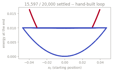
Each sample’s final energy against where it started: settled samples (the
active-set map dropped them) cluster near zero, the rest are still
oscillating when the batch hit max_steps.
import matplotlib.pyplot as plt
from nb_helpers import to_numpy

energy_host = to_numpy(energy)
terminated_host = to_numpy(terminated)

fig, ax = plt.subplots(figsize=(5, 3.2))
sc = ax.scatter(x0, energy_host, s=4, c=terminated_host, cmap="coolwarm_r")
ax.set_xlabel(r"$x_0$ (starting position)")
ax.set_ylabel("energy at the end")
ax.set_title(f"{int(terminated_host.sum()):,} / {n:,} settled -- hand-built loop")
fig.tight_layout()
plt.show()
simulate, run_until_done and this path#
simulate() is the call to reach for first. Given one kernel that
both advances the state and finishes its own samples, it runs
run_until_done() (an automatic number of steps per launch, picked
as the samples finish); given several, it composes exactly the loop above.
Composing Plan, GraphPipeline, ActiveSet and repeat_while yourself,
as here, is just as declarative, one level down, and stays the path for a loop
that does more than step: a step that alternates kernels, extra work between
compactions, or a larger graph the loop is one piece of.
Next#
Finished samples: compaction, reorder, and when not to – the active-set map on its own, with the numbers for when it pays.
deeper: Performance – the same loop shape, measured.