Where RAPTOR fits

See which kinds of GPU problems RAPTOR makes easy, and when another tool is the better choice — see the front page for the elevator pitch and the headline numbers; this page is the longer story: where RAPTOR sits, what it is not, and the same task in five tools, side by side.

The four principles

1. Efficient on the GPU. Whole pipelines replay as CUDA graphs — a GPU’s sequence of launches recorded once and replayed without re-issuing each one — so this class of problem makes full use of the hardware.

2. Written at the level of your application. A hawk kernel (a small GPU/CPU function, written once per sample) runs once per sample and declares, in its own signature, what each argument is (a per-sample state, a read-only table, an output); hawk works out the launch layout from that. CUDA C++, Warp, Numba and Triton still work right alongside it.

3. Differentiable, forward and backward. Every kernel’s reverse- and forward-mode derivatives are generated from the same source and run on the GPU or the CPU like the kernel itself.

4. Works with the code you already have. Arrays cross without copies through DLPack (a standard, framework-neutral way for one library to hand another an array without copying it), and a compiled kernel deploys into any program that reads its manifest.

The shape of it

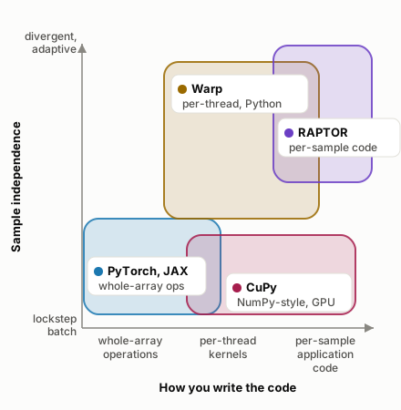
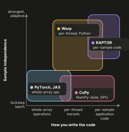
Tensor frameworks and CuPy write whole-array code for a lockstep batch; Warp and RAPTOR write closer to the thread or the sample and let samples branch and stop independently — the overlaps are complementary, not a ranking.

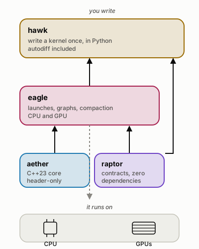
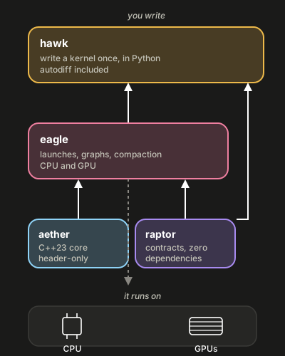
hawk is what you write; eagle runs it; aether and raptor are the two foundations underneath, and everything ultimately runs on CPU or GPUs — arrows follow the real dependencies, including raptor declared directly by both eagle and hawk.

aether lays out arrays and provides the device-safe vector-algebra vocabulary; eagle launches and captures what runs on top of it; raptor is the dependency-free foundation that defines the manifest and protocol contracts eagle and hawk both build to without depending on each other; hawk authors and compiles the kernels eagle deploys. A neural runtime built on this family is in development and not yet public.

Why it matters: keeping the GPU busy

Per-sample work is a demanding pattern for any parallel machine, and the arithmetic is rarely the hard part. The time tends to go to:

• launch overhead: one kernel launch per step, per stage, per sample group;

• host round-trips: the CPU checks “are we done yet?” between launches;

• dead lanes: in a vectorised batch, finished samples keep occupying the batch until the slowest one ends;

• two codebases: a GPU version and a CPU version that drift apart.

RAPTOR addresses each of these by construction:

• whole pipelines replay as captured CUDA graphs, removing the per-launch overhead;

• termination is decided on the device — each sample carries its own terminated flag and stops doing work once it’s set, removing the host round-trip;

• a finished sample does no further work, and active-set compaction (packing the still-running samples together so finished ones stop occupying GPU lanes) keeps the live samples packed, removing the dead lanes;

• one source serves both machines, so there is no second codebase to drift.

The point is to bring this class of problems toward the efficiency the hardware already delivers on dense tensor work, measured against the device’s own peak.

What happens to finished samples

A batch rarely finishes all at once: most samples stop at their own step, not the batch’s last one. What happens to a sample once it stops depends on how the loop is written. Masked array code keeps computing every sample every step, finished ones included, because the array doesn’t shrink. A hand-written per-thread kernel lets a finished thread exit, but the threads around it are grouped into warps of 32, and a warp only finishes once its slowest thread does — so an idle thread can still hold up its warp. eagle takes a third path: a finished sample leaves the active set, and the next launch covers only the samples still running, so the batch’s live set visibly shrinks as samples finish.

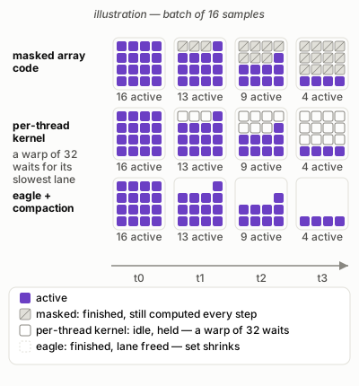
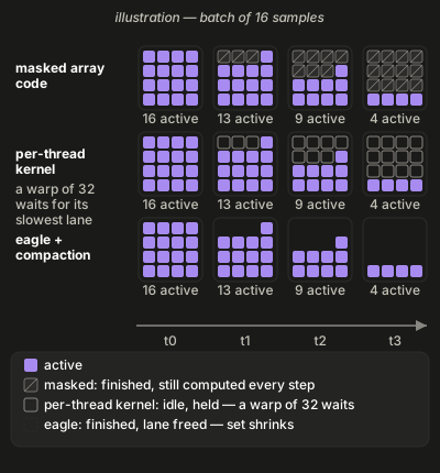
Illustration, not a measurement: a batch of 16 samples that stop at different steps, shown three ways.

The performance card has the real numbers, at real batch sizes, for the regime sketched above and several others — see Going deeper below for the worked-through figures.

What you write, side by side

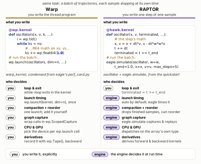
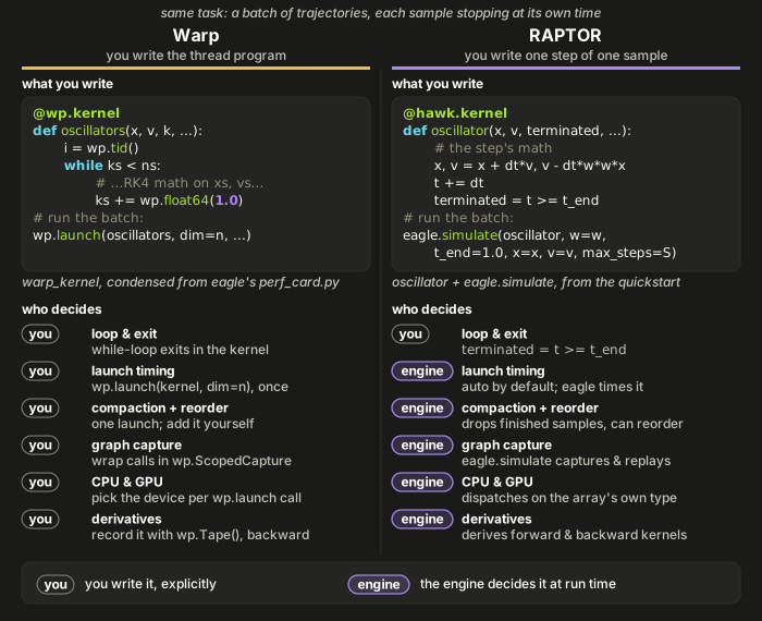
The same per-sample task written two ways: Warp’s explicit thread program next to a RAPTOR (hawk) kernel for one sample, with the run-time decisions each leaves to the author and each hands to the engine.

One level down, a kernel compiled elsewhere deploys through eagle.deploy(kernel) (or eagle.plan.auto, the same function) and loads by its manifest through eagle.registry.load_manifest. Full, runnable notebook.

What RAPTOR is for

• Many small problems, one per thread. Propagate ten thousand trajectories, integrate a batch of ODEs, step a population of agents. Each sample keeps its own state, takes its own branches and stops when it is done.

• One source, two machines. The same kernel compiles for a CUDA GPU or for CPU threads (parallelised with OpenMP, vectorised with SIMD — both standard ways to use multiple CPU cores and lanes at once). No second implementation to keep in sync, and the CPU build is the reference you test the GPU against.

• Kernels written in Python, compiled to native code. hawk traces a Python function into a typed intermediate representation (an internal, typed form of the code, not Python itself, that the compiler works from), derives its reverse- and forward-mode derivatives, and emits C++ for the GPU and the CPU.

• Launch overhead taken off the table. eagle captures whole pipelines as CUDA graphs and replays them, re-tuning launch geometry (how the work is split across GPU threads) between replays.

• Contracts, not glue. raptor’s manifest describes what a compiled kernel computes and how to call it, so a kernel built once can be deployed into any host that speaks the contract.

What RAPTOR is not

Not a deep-learning framework, not an autograd engine for whole programs, not a replacement for cuBLAS or cuDNN (NVIDIA’s own tuned dense-matrix and neural-network libraries) or any other tuned dense-tensor library. If your problem is one large dense tensor operation, the frameworks below will serve you better, and RAPTOR will happily consume their output.

Where we overlap, and what RAPTOR streamlines

Several jobs RAPTOR does are also done elsewhere. These are the ones where we think RAPTOR makes the path shorter or clearer:

You want to…	Common approaches	What RAPTOR adds
Write a custom GPU kernel from Python	write a CUDA C string for CuPy’s RawKernel, a Numba CUDA kernel, a Triton kernel (GPU-focused), or an NVIDIA Warp kernel (one source for CPU and CUDA)	write a typed Python function once; hawk emits it for the GPU and the CPU, with per-sample state and termination declared in the signature
Differentiate a custom kernel	write the backward pass yourself (e.g. a torch.autograd.Function or jax.custom_vjp), or use NVIDIA Warp, which differentiates its kernels in reverse mode	hawk derives both reverse- and forward-mode derivatives of the kernel itself, as kernels you can run anywhere the primal (the original kernel) runs
Run a batch where each sample branches and stops early	vectorise with vmap/masks, so finished samples keep occupying the batch	each sample owns its state and a terminated flag; finished samples stop working
Run the same algorithm on CPU and GPU	keep two code paths or two programming models (Warp is a notable exception)	one source, two compile targets, same results to within floating point; the CPU build doubles as the reference you test the GPU against
Remove launch overhead from a pipeline	use each framework’s own capture API (e.g. torch.cuda.graph, Warp’s ScopedCapture) around the calls	eagle captures and replays the pipeline, with microsecond-class re-tuning of launch sizes between replays
Pass arrays between libraries	DLPack, with the stream ordering left to you	DLPack with an explicit stream contract, ownership and access flags, and a certified interop matrix

hawk next to Warp

Warp and hawk both turn Python functions into CPU and GPU kernels, and both differentiate them. Each offers its own way of working:

• Termination lives in the signature. In hawk a sample’s terminated flag is part of the kernel’s declared vocabulary: the body writes the per-sample math, and finished samples stop committing results. In a thread-indexed kernel the same logic is explicit (a done flag, an early return, a guarded write-back), which gives full control over it; in hawk it follows from the signature.

• Authoring by declaration, not by indexing. A hawk kernel declares what each argument is (a per-sample state, a read-only table, a writable output, an accumulator), and hawk derives the indexing, the launch shape and the memory roles from those declarations.

• Kernels compose. Kernel kinds (named families of kernels that share a signature vocabulary) give a family of kernels a shared vocabulary; a kernel and its derived reverse- and forward-mode kernels are ordinary kernels you can deploy anywhere the primal (the original, undifferentiated kernel) runs; eagle captures several of them into one replayable graph; and raptor’s manifest lets a compiled kernel be dropped into another program.

Warp is the better choice when you want its built-in geometry, mesh and simulation library, or reverse-mode gradients of a whole simulation recorded on its tape (a runtime-recorded log of operations that a reverse-mode pass replays backward). The two work together: arrays pass between them zero-copy in both directions, with writes seen in the order they were issued — certified by three rows in raptor’s interoperability matrix (WP-IN-CUDA-ALIAS, WP-OUT-CUDA-ALIAS, STREAM-WARP-PRODUCER-ORDER — the matrix names and defines what each row id means). A side-by-side notebook — the same per-sample problem, with early termination, written in both and executed on the GPU, with the two results checked to agree — is 04_hawk_next_to_warp.

When another tool is the better choice

Tool	Choose it when…	Use it with RAPTOR by…
numpy	your data fits on the CPU and vectorised array code is fast enough	passing arrays in and out zero-copy (DLPack / array interface)
CuPy	you want numpy semantics on the GPU, or a hand-written CUDA kernel is fine	passing CuPy arrays zero-copy; RAPTOR kernels can run on CuPy’s stream
PyTorch	you train neural networks or need its ecosystem of models and operators	handing tensors over DLPack; a RAPTOR kernel can feed or consume a torch model
JAX	you want whole-program transformations (jit, grad, vmap) over array code, compiled through XLA (Google’s whole-program compiler)	exchanging arrays over DLPack (JAX support is on our roadmap; see below)
TensorFlow / Keras	you build and serve models in that ecosystem	exchanging tensors over DLPack (on our roadmap)
Numba	you want to JIT (just-in-time compile — turn a Python function into machine code the first time it runs) ordinary Python loops on the CPU, or write CUDA kernels in Python’s CUDA dialect	either side can consume the other’s arrays
Triton	you are writing high-performance dense GPU operators, especially for machine learning	composing at the array level
Warp	you want differentiable simulation kernels from Python for graphics, robotics or physics, with its rich built-in geometry and simulation library; it already offers one source for CPU and CUDA, reverse-mode kernel autodiff, CUDA-graph capture and DLPack	passing wp.arrays zero-copy both ways; see hawk next to Warp for what each makes easier

How they combine

Arrays cross the boundary through DLPack, zero-copy, with explicit stream ordering: the producer’s work is ordered before the consumer’s by a CUDA event, never by a device-wide synchronize. Every view reports who owns the memory, which library produced it, and whether it may be written.

• Supported today: CuPy, PyTorch and Warp, certified row by row in raptor’s interop matrix; numpy too, certified separately by an executable cuda-free dispatch test rather than a matrix row.

• Foreseen (same protocol, certification rows to come): JAX, TensorFlow/Keras and any other DLPack-capable library.

See raptor’s interoperability protocols for the full, cited statement of what is certified today versus foreseen, and eagle’s interoperability contract for the stream and lifetime rules.

Going deeper (optional)

The worked compaction numbers, and the same task written in five tools side by side — neither needed to follow the page above.

What compaction and eagle.simulate actually save

The performance card measures this on a development GPU (Quadro P2000), one million samples integrated for up to 1000 steps.

On a batch where samples finish at different times:

• the compacted graph takes 415 ms, against 625 ms for the identical workload run without compaction — what compaction itself saves at fixed work;

• an occasional physical reorder layered on top, opt-in and triggered only once the live samples have thinned and scattered, cuts that further to 279 ms;

• eagle.simulate — the policy that picks between these approaches at run time, so nobody has to choose by hand — reaches 156 ms on this same batch, ahead of NVIDIA Warp (609 ms), JAX (1.36 s), CuPy (7.38 s) and PyTorch (7.4 s) on this card.

On a batch where every sample runs the full 1000 steps instead, there is nothing to compact, and the plain graph is the better fit: 703 ms against 862 ms for the compacted graph, whose periodic active-set scan runs with no idle lanes left to recover. NVIDIA Warp’s per-thread kernel and eagle.simulate tie here (693 ms and 699 ms), and the two are level at N = 10,000 (7.22 ms against 7.22 ms) — worth knowing about. The card also lists the regimes where another approach is the better fit: on this FP64-weak development card the 8-thread CPU build is faster than every GPU arm on the dense batch (191 ms against 699 ms), and the same computation written as masked CuPy array code is the better fit when array-style code matters more than wall time.

Same task, five ways

Same task, five ways, measured by the RK7(8) card: two-body Kepler orbits (mu = 1, float64) from periapsis, a = 1, e uniform in [0, 0.9], random orientation; adaptive RKF7(8) (Fehlberg’s tableau, a mixed absolute/relative max-norm error control and a standard step-size controller). Largest batch shown: N = 1,000,000.

hawk + eagle

fact
lines (non-blank, non-comment)	22
what it brings here	the attempt is per-sample scalar code (22 lines with its launch; the kernel finishes its own samples), one kernel per attempt looped on the device: 23.5 s.
free from the same source	a CPU build from the same hawk kernel, with no second implementation to maintain, and the kernel’s own reverse- and forward-mode derivatives.

@hawk.kernel
def rkf78_attempt(t_final: Param, terminated: Terminated, s: Mutable[Vector[6]],
                  t: Mutable[Scalar], h: Mutable[Scalar],
                  n_acc: Mutable[Scalar], n_rej: Mutable[Scalar]):
    # One adaptive RKF7(8) attempt of this sample, with its step-size controller.
    s0 = s
    t0 = t
    last = h >= t_final - t0
    step = m.where(last, t_final - t0, h)  # clip onto the final time
    s8, err = rkf78_stages(s0, step, m.sqrt)
    ratio = error_ratio(s0, s8, err, abs, m.max)
    accept = ratio < 1.0
    expo = m.where(accept, EXP_ACCEPT, EXP_REJECT)
    h = step * m.min(MAX_SCALE, m.max(MIN_SCALE, SAFETY * ratio ** expo))
    s = m.where(accept, m.vec(s8), s0)
    t1 = m.where(accept, m.where(last, t_final, t0 + step), t0)
    t = t1
    n_acc = n_acc + m.where(accept, 1.0, 0.0)
    n_rej = n_rej + m.where(accept, 0.0, 1.0)
    terminated = t1 >= t_final  # the sample finishes itself

st.runner = eagle.until_done(eagle.deploy(rkf78_attempt), max_steps=MAX_ATTEMPTS,
                             t_final=T_FINAL, terminated=st.terminated,
                             **st.planes, **options)

CuPy

fact
lines (non-blank, non-comment)	25
what it brings here	array code in the NumPy style (25 lines), the control flow as masks over the batch: 182 s.
free from the same source	no second build and no gradient in this comparison; CuPy itself targets the GPU.

def cupy_attempt(s, t, h, n_acc, n_rej):
    """One masked RKF7(8) attempt over the whole batch (CuPy arrays)."""
    import cupy as cp

    running = t < T_FINAL
    last = h >= T_FINAL - t
    step = cp.where(last, T_FINAL - t, h)
    s8, err = rkf78_stages(s, step, cp.sqrt)
    ratio = error_ratio(s, s8, err, cp.abs, cp.maximum)
    accept = ratio < 1.0
    take = running & accept
    expo = cp.where(accept, EXP_ACCEPT, EXP_REJECT)
    scale = cp.clip(SAFETY * ratio ** expo, MIN_SCALE, MAX_SCALE)
    s = [cp.where(take, s8[d], s[d]) for d in range(6)]
    t = cp.where(take, cp.where(last, T_FINAL, t + step), t)
    h = cp.where(running, step * scale, h)
    return s, t, h, n_acc + take, n_rej + (running & ~accept), running


def cupy_run(st):
    p = st.planes
    s, t, h = [p[k] for k in STATE_NAMES], p["t"], p["h"]
    n_acc, n_rej = p["n_acc"], p["n_rej"]
    for _ in range(MAX_ATTEMPTS):
        s, t, h, n_acc, n_rej, running = cupy_attempt(s, t, h, n_acc, n_rej)
        if not bool(running.any()):
            break
    return s, t, h, n_acc, n_rej

PyTorch

fact
lines (non-blank, non-comment)	27
what it brings here	the same array formulation in PyTorch (27 lines), running where a PyTorch model already runs: 184 s.
free from the same source	gradients through torch.autograd, and the tensors run on CPU too (untested on this card).

def torch_attempt(s, t, h, n_acc, n_rej):
    """One masked RKF7(8) attempt over the whole batch (PyTorch tensors)."""
    import torch

    running = t < T_FINAL
    last = h >= T_FINAL - t
    step = torch.where(last, T_FINAL - t, h)
    s8, err = rkf78_stages(s, step, torch.sqrt)
    ratio = error_ratio(s, s8, err, torch.abs, torch.maximum)
    accept = ratio < 1.0
    take = running & accept
    expo = torch.where(accept, EXP_ACCEPT, EXP_REJECT)
    scale = torch.clamp(SAFETY * ratio ** expo, MIN_SCALE, MAX_SCALE)
    s = [torch.where(take, s8[d], s[d]) for d in range(6)]
    t = torch.where(take, torch.where(last, T_FINAL, t + step), t)
    h = torch.where(running, step * scale, h)
    return s, t, h, n_acc + take, n_rej + (running & ~accept), running


def torch_run(st):
    import torch

    with torch.inference_mode():
        p = st.planes
        s, t, h = [p[k] for k in STATE_NAMES], p["t"], p["h"]
        n_acc, n_rej = p["n_acc"], p["n_rej"]
        for _ in range(MAX_ATTEMPTS):
            s, t, h, n_acc, n_rej, running = torch_attempt(s, t, h, n_acc, n_rej)
            if not bool(running.any()):
                break
    return s, t, h, n_acc, n_rej

JAX

fact
lines (non-blank, non-comment)	25
what it brings here	writes the per-sample loop directly (25 lines) and compiles the whole batch into one executable: 40.2 s.
free from the same source	gradients through jax.grad, and the same code runs on a CPU backend (untested on this card).

def jax_integrate_fn():
    """jit(vmap(per-sample while loop)) over the initial states."""
    import jax
    import jax.numpy as jnp
    from jax import lax

    jax.config.update("jax_enable_x64", True)

    def one(s0):
        def cond(c):
            _, t, _, n_acc, n_rej = c
            return (t < T_FINAL) & (n_acc + n_rej < MAX_ATTEMPTS)

        def body(c):
            s, t, h, n_acc, n_rej = c
            last = h >= T_FINAL - t
            step = jnp.where(last, T_FINAL - t, h)
            s8, err = rkf78_stages(list(s), step, jnp.sqrt)
            ratio = error_ratio(list(s), s8, err, jnp.abs, jnp.maximum)
            accept = ratio < 1.0
            expo = jnp.where(accept, EXP_ACCEPT, EXP_REJECT)
            scale = jnp.clip(SAFETY * ratio ** expo, MIN_SCALE, MAX_SCALE)
            s = jnp.where(accept, jnp.stack(s8), s)
            t = jnp.where(accept, jnp.where(last, T_FINAL, t + step), t)
            return s, t, step * scale, n_acc + accept, n_rej + (1 - accept)

        init = (s0, jnp.float64(0.0), jnp.float64(H0), jnp.int64(0), jnp.int64(0))
        return lax.while_loop(cond, body, init)

    return jax.jit(jax.vmap(one))

Warp

fact
lines (non-blank, non-comment)	74
what it brings here	an explicit per-thread loop in a Python-embedded kernel language (74 lines, its own stages): 26.3 s.
free from the same source	reverse-mode gradients through wp.Tape, and a CPU device (untested on this card).

A = wp.constant(mat_a(*flat_a))
B = wp.constant(vec_s(*RK_B))
BE = wp.constant(vec_s(*RK_BE))

@wp.func
def rhs(s: vec6):
    r2 = s[0] * s[0] + s[1] * s[1] + s[2] * s[2]
    ir3 = f64(1.0) / (r2 * wp.sqrt(r2))
    return vec6(s[3], s[4], s[5], -s[0] * ir3, -s[1] * ir3, -s[2] * ir3)

@wp.kernel
def rkf78(x: wp.array(dtype=f64), y: wp.array(dtype=f64), z: wp.array(dtype=f64),
          vx: wp.array(dtype=f64), vy: wp.array(dtype=f64), vz: wp.array(dtype=f64),
          t_out: wp.array(dtype=f64), h_out: wp.array(dtype=f64),
          acc_out: wp.array(dtype=f64), rej_out: wp.array(dtype=f64),
          t_final: f64, rtol: f64, atol: f64, h0: f64, max_attempts: int):
    # one thread per sample: its whole adaptive loop to the final time
    i = wp.tid()
    s = vec6(x[i], y[i], z[i], vx[i], vy[i], vz[i])
    t = f64(0.0)
    h = h0
    n_acc = int(0)
    n_rej = int(0)
    while t < t_final and n_acc + n_rej < max_attempts:
        last = h >= t_final - t
        step = h
        if last:
            step = t_final - t
        k = mat_k()
        k0 = rhs(s)
        for d in range(6):
            k[0, d] = k0[d]
        for st in range(1, 13):
            si = s
            for j in range(st):
                if A[st, j] != f64(0.0):
                    for d in range(6):
                        si[d] = si[d] + step * A[st, j] * k[j, d]
            ks = rhs(si)
            for d in range(6):
                k[st, d] = ks[d]
        ratio = f64(0.0)
        s8 = s
        for d in range(6):
            acc = f64(0.0)
            err = f64(0.0)
            for st in range(13):
                acc = acc + B[st] * k[st, d]
                err = err + BE[st] * k[st, d]
            s8[d] = s[d] + step * acc
            sc = atol + rtol * wp.max(wp.abs(s8[d]), wp.abs(s[d]))
            ratio = wp.max(ratio, wp.abs(step * err) / sc)
        expo = f64(-0.125)
        if ratio < f64(1.0):
            expo = f64(-1.0 / 9.0)
        scale = wp.min(f64(5.0), wp.max(f64(0.2), f64(0.9) * wp.pow(ratio, expo)))
        if ratio < f64(1.0):
            s = s8
            t = t + step
            if last:
                t = t_final
            n_acc += 1
        else:
            n_rej += 1
        h = step * scale
    x[i] = s[0]
    y[i] = s[1]
    z[i] = s[2]
    vx[i] = s[3]
    vy[i] = s[4]
    vz[i] = s[5]
    t_out[i] = t
    h_out[i] = h
    acc_out[i] = f64(n_acc)
    rej_out[i] = f64(n_rej)

wp.launch(kernel, dim=n, inputs=[*s.planes.values(), T_FINAL, RTOL, ATOL, H0,
                                 MAX_ATTEMPTS], device="cuda:0")