Write one kernel. Run a million. Train it with PyTorch.

A ball thrown with air drag. Four short steps: write the physics for one sample, run it for a million, get its derivatives for free, then hand it to PyTorch to learn the drag coefficient from noisy landings.

Time: about 10 minutes · Runs on: CPU (GPU: the device switch below flips to it automatically) · You need: nothing but a Python environment.

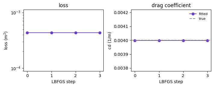
What you will build: a kernel you wrote, trained end to end against noisy data, in about 10 minutes.

This is also a self-contained notebook: download it or open it in Colab. Its first cell installs raptor-eagle/raptor-hawk for you if they aren’t already there.

Every cell below assumes the same small device switch every RAPTOR tutorial starts with — numpy on CPU, cupy on GPU, nothing imported unconditionally:

import numpy as np

try:
    import cupy as cp
    DEVICE = "gpu" if cp.cuda.runtime.getDeviceCount() > 0 else "cpu"
except Exception:
    DEVICE = "cpu"
xp = cp if DEVICE == "gpu" else np

1. Write one sample’s kernel

A hawk kernel is a plain Python function: it reads the planes it declares and writes the ones it owns. r/v are this ball’s position and velocity — Mutable, because the kernel updates them. Read one like any local variable (you get the value from when this launch began, until the kernel itself assigns a new one); write the result back by assigning to the same name. cd is the drag coefficient, one Scalar per sample; dt/g are Params, one value shared by everyone. terminated = ... is the stop rule: once a ball’s height goes below zero, it’s done.

One call, eagle.simulate, runs it: pass the kernel’s arguments as you would call it, plain floats in, one throw out.

import hawk
from hawk import Mutable, Param, Scalar, Terminated, Vector
from hawk.math import norm, vec
import eagle


@hawk.kernel
def flight(cd: Scalar, dt: Param, g: Param, terminated: Terminated,
           r: Mutable[Vector[3]], v: Mutable[Vector[3]]):
    a = vec(0.0, 0.0, -g) - cd * norm(v) * v
    v = v + dt * a
    r = r + dt * v
    terminated = r[2] < 0


one = eagle.simulate(
    flight,
    cd=0.004, dt=0.01, g=9.81,
    r=xp.array([0.0, 0.0, 1.0]), v=xp.array([20.0, 0.0, 15.0]),
    max_steps=2000,
)
print(one.status, one.steps, one.r)
# finished 320 [53.08994129  0.         -0.05716388]

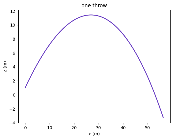
What just happened:

• flight is one sample’s physics: gravity plus quadratic drag, a semi-implicit Euler step.

• terminated marked this sample done at step 320, the step its height first went below zero — eagle.simulate stopped there instead of running to max_steps.

• one.r is the landing position: about 53 m downrange.

2. Run a lot of them

The same call, with arrays instead of plain numbers — cd now needs one value per sample too. CPU defaults to 100,000 throws so this stays fast without a GPU; the notebook sets n = 1_000_000 once DEVICE == "gpu". The full random batch (speeds, elevations, headings) is in the notebook; this page only quotes the call and its result.

n = 100_000  # 1_000_000 once a GPU is visible (see the notebook's device switch)
r, v = ..., ...  # n throws, random speeds and angles -- see the notebook
many = eagle.simulate(
    flight, cd=xp.full(n, 0.004), dt=0.01, g=9.81, r=r, v=v,
    max_steps=2000,
)
print(f"{many.finished.sum():,} / {n:,} finished, {many.report.launches} launches, "
      f"{many.wall_s * 1e3:.1f} ms (on the machine that built this page)")
# 100,000 / 100,000 finished, 8 launches, … ms (on the machine that built this page)

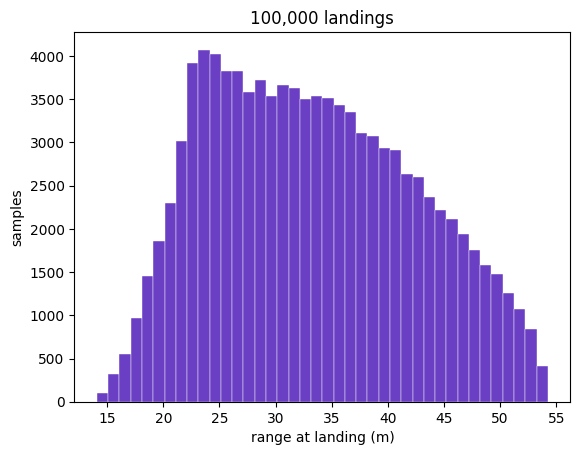
What just happened:

• Every sample ran the same kernel; each stopped on its own step, and the finished ones stopped costing launches.

• 100,000 throws took 8 launches, not 100,000 — launches are batched, not one per sample or one per step.

• The histogram is this run’s own throws: a spread of ranges from a spread of speeds and angles.

3. Get derivatives

eagle.frameworks.torch.function wraps a kernel as a torch.autograd.Function: forward runs the kernel, backward runs the derived reverse-mode kernel — nothing is taped. This uses flight_step, the one-step kernel from eagle’s own torch training tutorial (separate in- and next-state planes, the shape torch.autograd.Function wants). torch.autograd.gradcheck compares it against finite differences.

from eagle.frameworks import torch as eagle_torch


@hawk.kernel
def flight_step(
    r: Vector[3], v: Vector[3], cd: Scalar, dt: Param, g: Param,
    terminated: Terminated, r_next: Mutable[Vector[3]], v_next: Mutable[Vector[3]],
):
    a = vec(0.0, 0.0, -g) - cd * norm(v) * v
    v_next = v + dt * a
    r_next = r + dt * v_next


step = eagle_torch.function(flight_step, wrt=("r", "v", "cd"))

m = 8
r = torch.randn(3, m, dtype=torch.float64, requires_grad=True)
v = torch.randn(3, m, dtype=torch.float64, requires_grad=True)
cd = torch.rand(m, dtype=torch.float64, requires_grad=True)
landed = torch.zeros(m, dtype=torch.bool)
landed[[2, 5]] = True  # two of the eight samples already landed

ok = torch.autograd.gradcheck(
    lambda r, v, cd: step(r, v, cd, 0.05, 9.81, landed),
    (r, v, cd), check_forward_ad=True, check_batched_grad=False,
)
print("gradcheck:", ok)
# gradcheck: True

What just happened:

• step is flight_step’s derived reverse- and forward-mode kernel, compiled the first time it ran.

• gradcheck matches both against finite differences: True.

• A terminated sample gets exactly zero gradient — it never corrects a later step.

4. Hand it to PyTorch

many.r from step 2 is a plain NumPy array on CPU (a CuPy one on GPU). The rest of this step crosses it into torch, builds a tiny model around step from step 3, and fits the drag coefficient to noisy “observed” landings.

Cross it into torch. torch.from_dlpack crosses an array into torch without copying it, when the backing memory supports that.

landed_torch = torch.from_dlpack(many.r)
same_memory = np.shares_memory(np.asarray(many.r), landed_torch.numpy())
print("shares memory on this machine:", same_memory)
# shares memory on this machine: True

A CUDA array crossing this way is raptor’s certified T-IN-CUDA-ALIAS row — always zero-copy; a plain NumPy one isn’t a certified crossing at all, so the notebook checks rather than assumes it.

Build a tiny model around step. Ballistic unrolls step from step 3 over a flight; its one learned value is log(cd), not cd itself, so training can never push the drag coefficient negative (see the notebook for the class).

Make up something to fit. Run Ballistic with the true drag coefficient to get a batch of clean landings, then add a little noise — that noisy batch is what the model below has to explain (random throws and the noise draw are in the notebook):

truth = Ballistic(0.004)(r0, v0)  # r0, v0: 128 random throws -- see the notebook
observed = truth + 0.02 * torch.randn(truth.shape, dtype=torch.float64)
print(f"{observed.shape[-1]} synthetic throws, noise std 0.02 m")
# 128 synthetic throws, noise std 0.02 m

Train it. The same story as eagle’s own torch tutorial, starting from a guess five times too large, fit with torch.optim.LBFGS:

model = Ballistic(cd_guess=0.02)
optimizer = torch.optim.LBFGS(
    model.parameters(), max_iter=20, line_search_fn="strong_wolfe")
for epoch in range(4):
    optimizer.step(closure)  # closure() re-evaluates the loss and calls .backward()
print(f"learned cd = {model.log_cd.exp().item():.6f} /m (true 0.004 /m)")
# learned cd = 0.003999 /m (true 0.004 /m)

What just happened:

• step’s derived gradient (from step 3) is what loss.backward() used to update the model’s one parameter — no finite differences in the training loop.

• L-BFGS found the true drag coefficient, 0.004 /m, from noisy landings in a handful of evaluations.

• The full model (the Ballistic class, the noisy “observed” data, the plotting) is in the notebook — this page only quotes the fit itself.

One loose end. Inside Ballistic, each step works out is_landed = r[2] < 0.0 by hand and uses torch.where to freeze a landed sample’s state — the same idea as terminated from step 1, just worked out again here because step() hands back the next position and velocity but not its own stop decision. A later version of step() may return that decision directly, so the loop could reuse it instead of recomputing it.

Where to next

• hawk — write your own kernels and vocabularies.

• eagle — make them fast: graphs, compaction, profiling.

• aether — the C++ underneath, if you need it directly.

• raptor — plug a new engine or framework into the contracts this page used.

deeper: where RAPTOR fits has the full four-part story.